Numerical Analysis
Overview
The analysis package is the parent package for algorithms dealing with real-valued functions of one real variable. It contains dedicated sub-packages providing numerical root-finding, integration, interpolation and differentiation. It also contains a polynomials sub-package that considers polynomials with real coefficients as differentiable real functions.
Functions interfaces are intended to be implemented by user code to represent their domain problems. The algorithms provided by the library will then operate on these function to find their roots, or integrate them, or … Functions can be multivariate or univariate, real vectorial or matrix valued, and they can be differentiable or not.
Error handling
For user-defined functions, when the method encounters an error during evaluation, users must use their own unchecked exceptions. The following example shows the recommended way to do that, using root solving as the example (the same construct should be used for ODE integrators or for optimizations).
private static class LocalException extends RuntimeException {

   // the x value that caused the problem
   private final double x;

   public LocalException(double x) {
     this.x = x;
   }

   public double getX() {
     return x;
   }

 }

 private static class MyFunction implements UnivariateFunction {
   public double value(double x) {
     double y = hugeFormula(x);
     if (somethingBadHappens) {
       throw new LocalException(x);
     }
     return y;
   }
 }

 public void compute() {
   try {
     solver.solve(maxEval, new MyFunction(a, b, c), min, max);
   } catch (LocalException le) {
     // retrieve the x value
   }
 }
As shown in this example the exception is really something local to user code and there is a guarantee Hipparchus will not mess with it. The user is safe.
Root-finding
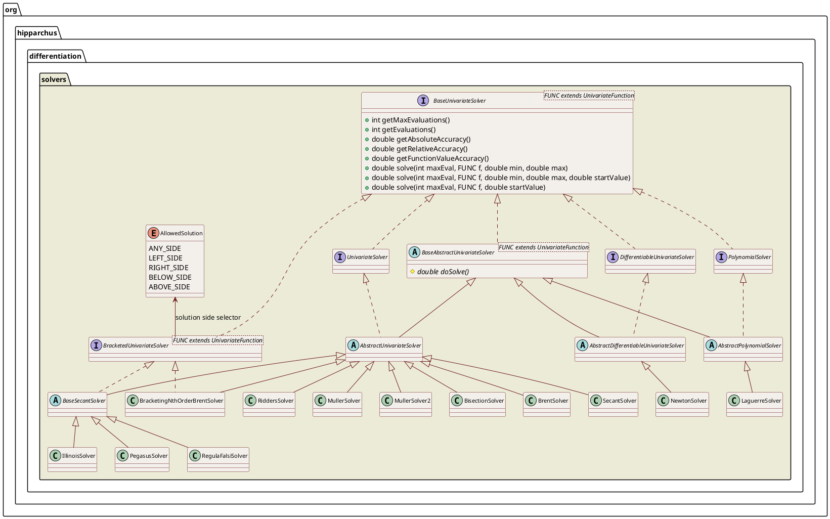
UnivariateSolver, UnivariateDifferentiableSolver and PolynomialSolver provide means to find roots of univariate real-valued functions, differentiable univariate real-valued functions, and polynomial functions respectively. A root is the value where the function takes the value 0. Hipparchus includes implementations of the several root-finding algorithms:
| Root solvers | ||||
|---|---|---|---|---|
| Name | Function type | Convergence | Needs initial bracketing | Bracket side selection |
| Bisection | univariate real-valued functions | linear, guaranteed | yes | yes |
| Brent-Dekker | univariate real-valued functions | super-linear, guaranteed | yes | no |
| bracketing n | univariate real-valued functions | variable order, guaranteed | yes | yes |
| Illinois Method | univariate real-valued functions | super-linear, guaranteed | yes | yes |
| Laguerre's Method | polynomial functions | cubic for simple root, linear for multiple root | yes | no |
| Muller's Method using bracketing to deal with real-valued functions | univariate real-valued functions | quadratic close to roots | yes | no |
| Muller's Method using modulus to deal with real-valued functions | univariate real-valued functions | quadratic close to root | yes | no |
| Newton-Raphson's Method | differentiable univariate real-valued functions | quadratic, non-guaranteed | no | no |
| Pegasus Method | univariate real-valued functions | super-linear, guaranteed | yes | yes |
| Regula Falsi (false position) Method | univariate real-valued functions | linear, guaranteed | yes | yes |
| Ridder's Method | univariate real-valued functions | super-linear | yes | no |
| Secant Method | univariate real-valued functions | super-linear, non-guaranteed | yes | no |
Some algorithms require that the initial search interval bracket the root (i.e. the function values at interval end points have opposite signs). Some algorithms preserve bracketing throughout computation and allow the user to specify which side of the convergence interval to select as the root. It is also possible to force a side selection after a root has been found even for algorithms that do not provide this feature by themselves. This is useful for example in sequential search, for which a new search interval is started after a root has been found in order to find the next root. In this case, the user must select a side to ensure that the loop does not get stuck on one root, always returning the same solution without making any progress.
There are numerous non-obvious traps and pitfalls in root-finding. First, the usual disclaimers due to the way real world computers calculate values apply. If the computation of the function provides numerical instabilities, for example due to bit cancellation, the root finding algorithms may behave badly and fail to converge or even return bogus values. There will not necessarily be an indication that the computed root is way off the true value. Secondly, the root-finding problem itself may be inherently ill-conditioned. There is a “domain of indeterminacy”, the interval for which the function has near zero absolute values around the true root, which may be large. Even worse, small problems like roundoff error may cause the function value to “numerically oscillate” between negative and positive values. This may again result in roots way off the true value, without indication. There is not much a generic algorithm can do if ill-conditioned problems are met. A way around this is to transform the problem in order to get a better-conditioned function. Proper selection of a root-finding algorithm and its configuration parameters requires knowledge of the analytical properties of the function under analysis and numerical analysis techniques. Users are encouraged to consult a numerical analysis text (or a numerical analyst) when selecting and configuring a solver.
In order to use the root-finding features, first a solver object must be created by calling its constructor, often providing relative and absolute accuracy. Using a solver object, roots of functions are easily found using the solve methods. These methods take a maximum iteration count maxEval, a function f, and either two domain values, min and max, or a startValue as parameters. If the maximum number of iterations is exceeded, non-convergence is assumed and a MathIllegalStateException exception is thrown. A suggested value is 100, which should be plenty, given that a bisection algorithm can't get any more accurate after 52 iterations because of the number of mantissa bits in a double precision floating point number. If a number of ill-conditioned problems are to be solved, this number can be decreased in order to avoid wasting time. Bracketed solvers also take an allowed solution enum parameter to specify which side of the final convergence interval should be selected as the root. It can be ANY_SIDE, LEFT_SIDE, RIGHT_SIDE, BELOW_SIDE or ABOVE_SIDE. Left and right are used to specify the root along the function parameter axis while below and above refer to the function value axis. The solve methods compute a value \(c\) such that:
- \(f(c) = 0.0\) (see “function value accuracy”)
- \(min \le c \le max \) (except for the secant method, which may find a solution outside the interval)
Typical usage:
UnivariateFunction function = ...; // some user defined function object
final double relativeAccuracy = 1.0e-12;
final double absoluteAccuracy = 1.0e-8;
final int    maxOrder         = 5;
UnivariateSolver solver = new BracketingNthOrderBrentSolver(relativeAccuracy, absoluteAccuracy, maxOrder);
double c = solver.solve(100, function, 1.0, 5.0, AllowedSolution.LEFT_SIDE);
Force bracketing, by refining a base solution found by a non-bracketing solver:
UnivariateFunction function = ...; // some user defined function object
final double relativeAccuracy = 1.0e-12;
final double absoluteAccuracy = 1.0e-8;
UnivariateSolver nonBracketing = new BrentSolver(relativeAccuracy, absoluteAccuracy);
double baseRoot = nonBracketing.solve(100, function, 1.0, 5.0);
double c = UnivariateSolverUtils.forceSide(100, function,
                                           new PegasusSolver(relativeAccuracy, absoluteAccuracy),
                                           baseRoot, 1.0, 5.0, AllowedSolution.LEFT_SIDE);
The BrentSolver uses the Brent-Dekker algorithm which is fast and robust. If there are multiple roots in the interval, or there is a large domain of indeterminacy, the algorithm will converge to a random root in the interval without indication that there are problems.
Interestingly, the examined text book implementations all disagree in details of the convergence criteria. Also each implementation had problems for one of the test cases, so the expressions had to be fudged further. Don't expect to get exactly the same root values as for other implementations of this algorithm.
The BracketingNthOrderBrentSolver uses an extension of the Brent-Dekker algorithm which uses inverse nth order polynomial interpolation instead of inverse quadratic interpolation, and which allows selection of the side of the convergence interval for result bracketing. This is now the recommended algorithm for most users since it has the largest order, doesn't require derivatives, has guaranteed convergence and allows result bracket selection.
The SecantSolver uses a straightforward secant algorithm which does not bracket the search and therefore does not guarantee convergence. It may be faster than Brent on some well-behaved functions.
The RegulaFalsiSolver is variation of secant preserving bracketing, but then it may be slow, as one end point of the search interval will become fixed after and only the other end point will converge to the root, hence resulting in a search interval size that does not decrease to zero.
The IllinoisSolver and PegasusSolver are well-known variations of regula falsi that fix the problem of stuck end points by slightly weighting one endpoint to balance the interval at next iteration. Pegasus is often faster than Illinois. Pegasus may be the algorithm of choice for selecting a specific side of the convergence interval.
The BisectionSolver is included for completeness and for establishing a fallback in cases of emergency. The algorithm is simple, most likely bug free and guaranteed to converge even in very adverse circumstances which might cause other algorithms to malfunction. The drawback is of course that it is also guaranteed to be slow.
The UnivariateSolver interface exposes many properties to control the convergence of a solver. The accuracy properties are set at solver instance creation and cannot be changed afterwards, there are only getters to retrieve their values, no setters are available.
| Property | Purpose |
|---|---|
| Absolute accuracy | The Absolute Accuracy is (estimated) maximum difference between the computed root and the true root of the function. This is what most people think of as “accuracy” intuitively. The default value is chosen as a sane value for most real-world problems, for roots in the range from -100 to +100. For accurate computation of roots near zero, in the range form -0.0001 to +0.0001, the value may be decreased. For computing roots much larger in absolute value than 100, the default absolute accuracy may never be reached because the given relative accuracy is reached first. |
| Relative accuracy | The Relative Accuracy is the maximum difference between the computed root and the true root, divided by the maximum of the absolute values of the numbers. This accuracy measurement is better suited for numerical calculations with computers, due to the way floating point numbers are represented. The default value is chosen so that algorithms will get a result even for roots with large absolute values, even while it may be impossible to reach the given absolute accuracy. |
| Function value accuracy | This value is used by some algorithms in order to prevent numerical instabilities. If the function is evaluated to an absolute value smaller than the Function Value Accuracy, the algorithms assume they hit a root and return the value immediately. The default value is a “very small value”. If the goal is to get a near zero function value rather than an accurate root, computation may be sped up by setting this value appropriately. |
Interpolation
A UnivariateInterpolator is used to find a univariate real-valued function f which for a given set of ordered pairs \((x_i,y_i)\) yields \(f(x_i)=y_i\) to the best accuracy possible. The result is provided as an object implementing the Univariate interface. It can therefore be evaluated at any point, including point not belonging to the original set. Currently, only an interpolator for generating natural cubic splines and a polynomial interpolator are available. There is no interpolator factory, mainly because the interpolation algorithm is more determined by the kind of the interpolated function rather than the set of points to interpolate. There aren't currently any accuracy controls either, as interpolation accuracy is in general determined by the algorithm.
Typical usage:
double x[] = { 0.0, 1.0, 2.0 };
double y[] = { 1.0, -1.0, 2.0};
UnivariateInterpolator interpolator = new SplineInterpolator();
UnivariateFunction function = interpolator.interpolate(x, y);
double interpolationX = 0.5;
double interpolatedY = function.value(x);
System.out.println("f(" + interpolationX + ") = " + interpolatedY);
A natural cubic spline is a function consisting of a polynomial of third degree for each subinterval determined by the x-coordinates of the interpolated points. A function interpolating N value pairs consists of N-1 polynomials. The function is continuous, smooth and can be differentiated twice. The second derivative is continuous but not smooth. The x values passed to the interpolator must be ordered in ascending order. It is not valid to evaluate the function for values outside the range \(x_0…x_N\).
The polynomial function returned by the Neville's algorithm is a single polynomial guaranteed to pass exactly through the interpolation points. The degree of the polynomial is the number of points minus 1 (i.e. the interpolation polynomial for a three points set will be a quadratic polynomial). Despite the fact the interpolating polynomials is a perfect approximation of a function at interpolation points, it may be a loose approximation between the points. Due to Runge's phenomenom the error can get worse as the degree of the polynomial increases, so adding more points does not always lead to a better interpolation.
Loess (or Lowess) interpolation is a robust interpolation useful for smoothing univariate scaterplots. It has been described by William Cleveland in his 1979 seminal paper Robust Locally Weighted Regression and Smoothing Scatterplots. This kind of interpolation is computationally intensive but robust.
]Microsphere interpolation]((../apidocs/org/hipparchus/analysis/interpolation/MicrosphereProjectionI,terpolator.html)) is a robust multidimensional interpolation algorithm. It has been described in William Dudziak's MS thesis.
Hermite interpolation is an interpolation method that can use derivatives in addition to function values at sample points. The HermiteInterpolator class implements this method for vector-valued functions. The sampling points can have any spacing (there are no requirements for a regular grid) and some points may provide derivatives while others don't provide them (or provide derivatives to a smaller order). Points are added one at a time, as shown in the following example:
HermiteInterpolator interpolator = new HermiteInterpolator;
// at x = 0, we provide both value and first derivative
interpolator.addSamplePoint(0.0, new double[] { 1.0 }, new double[] { 2.0 });
// at x = 1, we provide only function value
interpolator.addSamplePoint(1.0, new double[] { 4.0 });
// at x = 2, we provide both value and first derivative
interpolator.addSamplePoint(2.0, new double[] { 5.0 }, new double[] { 2.0 });
// should print "value at x = 0.5: 2.5625"
System.out.println("value at x = 0.5: " + interpolator.value(0.5)[0]);
// should print "derivative at x = 0.5: 3.5"
System.out.println("derivative at x = 0.5: " + interpolator.derivative(0.5)[0]);
// should print "interpolation polynomial: 1 + 2 x + 4 x^2 - 4 x^3 + x^4"
System.out.println("interpolation polynomial: " + interpolator.getPolynomials()[0]);
A BivariateGridInterpolator is used to find a bivariate real-valued function f which for a given set of tuples \((x_i,y_j,f_{ij})\) yields \(f(x_i,y_j)=f_{ij}\) to the best accuracy possible. The result is provided as an object implementing the BivariateFunction interface. It can therefore be evaluated at any point, including a point not belonging to the original set. The arrays \(x_i\) and \(y_j\) must be sorted in increasing order in order to define a two-dimensional grid.
In bicubic interpolation, the interpolation function is a 3rd-degree polynomial of two variables. The coefficients are computed from the function values sampled on a grid, and if available from the values of the partial derivatives of the function at those grid points. For two-dimensional data sampled on a grid with derivatives available, the BicubicInterpolator computes a bicubic interpolating function. For two-dimensional data sampled on a grid without derivatives available, the PiecewiseBicubicSplineInterpolator computes a piecewise bicubic interpolating function.
A TrivariateGridInterpolator is used to find a trivariate real-valued function f which for a given set of tuples \((x_i,y_j,z_k, f_{ijk})\) yields \(f(x_i,y_j,z_k)=f_{ijk}\) to the best accuracy possible. The result is provided as an object implementing the TrivariateFunction interface. It can therefore be evaluated at any point, including a point not belonging to the original set. The arrays \(x_i\), \(y_j\) and \(z_k\) must be sorted in increasing order in order to define a three-dimensional grid.
In tricubic interpolation, the interpolation function is a 3rd-degree polynomial of three variables. The coefficients are computed from the function values sampled on a grid, as well as the values of the partial derivatives of the function at those grid points. From three-dimensional data sampled on a grid, the TricubicSplineInterpolator computes a tricubic interpolating function.
Integration
A UnivariateIntegrator provides the means to numerically integrate univariate real-valued functions.
Integration is also available as part of DerivativeStructure.
Hipparchus includes implementations of the following integration algorithms:
Polynomials
The org.hipparchus.analysis.polynomials package provides real coefficients polynomials.
The PolynomialFunction class is the most general one, using traditional coefficients arrays. The PolynomialsUtils utility class provides static factory methods to build Chebyshev, Hermite, Jacobi, Laguerre and Legendre polynomials. Coefficients are computed using exact fractions so these factory methods can build polynomials up to any degree.
Differentiation
The org.hipparchus.analysis.differentiation package provides a general-purpose differentiation framework.
Automated differentiation using DerivativeStructure
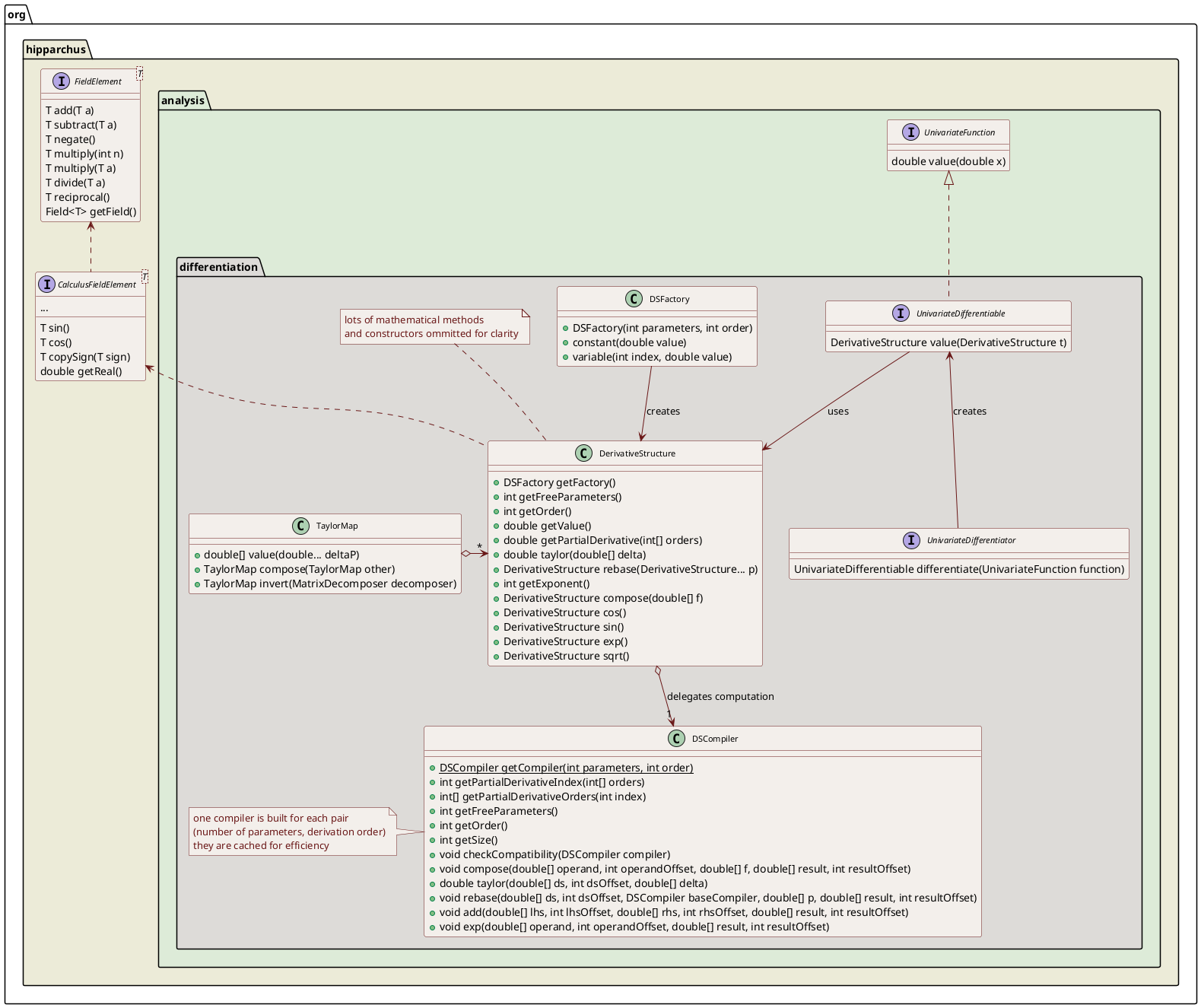
The core class is DerivativeStructure which holds the value and the differentials of a function. This class handles some arbitrary number of free parameters and arbitrary derivation order. It is used both as the input and the output type for the UnivariateDifferentiableFunction interface. Any differentiable function should implement this interface.
The main idea behind the DerivativeStructure class is that it can be used almost as a number (i.e. it can be added, multiplied, its square root can be extracted or its cosine computed… However, in addition to computed the value itself when doing these computations, the partial derivatives are also computed alongside. This is an extension of what is sometimes called Rall's numbers. This extension is described in Dan Kalman's paper Doubly Recursive Multivariate Automatic Differentiation, Mathematics Magazine, vol. 75, no. 3, June 2002. Rall's numbers only hold the first derivative with respect to one free parameter whereas Dan Kalman's derivative structures hold all partial derivatives up to any specified order, with respect to any number of free parameters. Rall's numbers therefore can be seen as derivative structures for order one derivative and one free parameter, and primitive real numbers can be seen as derivative structures with zero order derivative and no free parameters.
The workflow of computation of a derivatives of an expression \(y=f(x)\) is as follows. First we configure a factory with the number of free parameters and the derivation order we want to use throughout the computation. Then we use it to create variables (one for each of the free parameters, here only one since the single free parameter is \(x\)) and constants that will be used for the rest of the computation. Variables, constants, intermediate values and final results will all be instances of DerivativeStructure. We compute \(y=f(x)\) normally by using all these instances just as we would use regular numbers (apart from the fact we must write things like a.add(b) instead of \(a + b\) as the Java languages does not support operator overriding). At the end, we extract from \(y\) the value and the derivatives we want. As we have specified \(3^\mathrm{rd}\) order when we built \(\), we can retrieve the derivatives up to \(3^\mathrm{rd}\) order from \(y\). The following example shows that:
int params = 1;
int order = 3;
DSFactory factory = new DSFactory(params, order);

double xRealValue = 2.5;
DerivativeStructure x = factory.variable(0, xRealValue);
DerivativeStructure y = f(x);
System.out.println("y    = " + y.getValue();
System.out.println("y'   = " + y.getPartialDerivative(1);
System.out.println("y''  = " + y.getPartialDerivative(2);
System.out.println("y''' = " + y.getPartialDerivative(3);
with for example this definition for the \(f(x) = \cos(1+x)\) function:
public DerivativeStructure f(DerivativeStructure x) {
    return x.add(1).cos();
}
In fact, there are no special provisions for variables in the framework, so neither \(x\) nor \(y\) are considered to be variables per se. They are both considered to be functions and to depend on implicit free parameters which are represented only by indices in the framework. The \(x\) instance above is there considered by the framework to be a function of free parameter \(p_0\) at index 0, and as \(y\) is computed from \(x\) it is the result of a functions composition and is therefore also a function of this \(p_0\) free parameter. The \(p_0\) is not represented by itself, it is simply defined implicitly by the 0 index above. This index is the first argument in the call to the variable factory method to create the \(x\) instance. What this factory method means is that we built \(x\) as a function that depends on one free parameter only, that can be differentiated up to order 3 (as specified when the factory was configured), and which correspond to an identity function with respect to implicit free parameter number 0 (first factory method argument set to 0), with current value equal to 2.5 (second factory method argument set to 2.5). This specific factory method defines identity functions, and identity functions are the trick we use to represent variables (there are of course other constructors, for example to build constants or functions from all their derivatives if they are known beforehand). From the user point of view, the \(x\) instance can be seen as the \(x\) variable, but it is really the identity function applied to free parameter number 0. As the identity function, it has the same value as its parameter, its first derivative is 1.0 with respect to this free parameter, and all its higher order derivatives are 0.0. This can be checked by calling the getValue() or getPartialDerivative() methods on \(x\).
When we compute \(y\) from this setting, what we really do is chain \(f\) after the identity function, so the net result is that the derivatives are computed with respect to the indexed free parameters (i.e. only free parameter number 0 here since there is only one free parameter) of the identity function \(x\). Going one step further, if we compute \(z = g(y)\), we will also compute \(z\) as a function of the initial free parameter. The very important consequence is that if we call z.getPartialDerivative(1), we will not get the first derivative of \(g\) with respect to \(y\), but with respect to the free parameter \(p_0\): the derivatives of \(g\) and \(f\) will be chained together automatically, without user intervention.
This design choice is a very classical one in many algorithmic differentiation frameworks, either based on operator overloading (like the one we implemented here) or based on code generation. It implies the user has to bootstrap the system by providing initial derivatives, and this is essentially done by setting up identity function, i.e. functions that represent the variables themselves and have only unit first derivative.
This design also allows a very interesting feature which can be explained with the following example. Suppose we have a two-argument function \(f\) and a one-argument function \(g\). If we compute \(g(f(x, y))\) with \(x\) and \(y\) be two variables, we want to be able to compute the partial derivatives \(\partial g / \partial x\), \(\partial g / \partial y\), \(\partial^2 g / \partial x^2\), \(\partial^2 g / \partial x\partial y\) and \(\partial^2 g / \partial y^2\). This does make sense since we combined the two functions, and it does make sense despite \(g\) is a one argument function only. In order to do this, we simply set up \(x\) as an identity function of an implicit free parameter \(p_0\) and \(y\) as an identity function of a different implicit free parameter \(p_1\) and compute everything directly. In order to be able to combine everything, however, both \(x\) and \(y\) must be built with the appropriate dimensions, so the factory used to create them must have been configured to managed two parameters. The \(x\) instance will be created by calling the factory method variable with the first parameter set to 0, whereas the \(y\) instance will be created by calling the factory method variable with the first parameter set to 1, so they refer to different parameters. Here is how we do this (note that getPartialDerivative is a variable arguments method which take as arguments the derivation order with respect to all free parameters, i.e. the first argument is derivation order with respect to free parameter 0 and the second argument is derivation order with respect to free parameter 1):
int params = 2;
int order = 2;
DSFactory factory = new DSFactory(params, order);

double xRealValue =  2.5;
double yRealValue = -1.3;
DerivativeStructure x = factory.variable(0, xRealValue);
DerivativeStructure y = factory.variable(1, yRealValue);
DerivativeStructure f = DerivativeStructure.hypot(x, y);
DerivativeStructure g = f.log();
System.out.println("g        = " + g.getValue();
System.out.println("dg/dx    = " + g.getPartialDerivative(1, 0);
System.out.println("dg/dy    = " + g.getPartialDerivative(0, 1);
System.out.println("d2g/dx2  = " + g.getPartialDerivative(2, 0);
System.out.println("d2g/dxdy = " + g.getPartialDerivative(1, 1);
System.out.println("d2g/dy2  = " + g.getPartialDerivative(0, 2);
It is possible to integrate or differentiate a DerivativeStructure. When integrating, the integration constants are systematically set to zero. When differentiating, the resulting derivative structure is truncated to the initial order (i.e. a derivative structure up to order 3 differentiated twice will still be of order 3, and the two highest order terms (4 and 5) will be dropped.
If a function \(f\) is a function of \(n\) independent parameters \(p_0, p_1, \ldots p_{n-1}\), then it can be computed as a DerivativeStructure with \(n\) parameters. If however, in another part of the computation the parameters are themselves considered to be functions of \(m\) more base variables \(p_0 = p_0(q_0, q_1, \ldots q_{m-1})\), \(p_1 = p_1(q_0, q_1, \ldots q_{m-1})\), … \(p_{n-1} = p_{n-1}(q_0, q_1, \ldots q_{m-1})\), then it is possible to rebase the initial DerivativeStructure by providing the intermediate variables \(p_i\) as DerivativeStructure with \(m\) parameters. The result will be a DerivativeStructure with \(m\) parameters representing \(f(q_0, q_1, \ldots q_{m-1})\). When rebasing, the number of intermediate variables \(p_i\) provided must match the number \(n\) of parameters of the initial DerivativeStructure, and the derivation orders must all match.
The TaylorMap class is a container that gather several DerivativeStructure and one evaluation point \((p_0, p_1, \ldots p_{n-1})\) to represent a vector-valued function. Taylor maps can be evaluated at points close to the central evaluation point by providing the offsets \((\Delta p_0, \Delta p_1, \ldots \Delta p_{n-1})\). They can be composed with other Taylor maps, which corresponds to calling rebase on all vector components, provided that the number of functions of the inner map is equal to the number of parameters of the outer map. If a Taylor map is square (i.e. if its number of parameters is equal to its number of functions) and if its first order derivatives are non-singular, then it can be inverted. Taylor map inversion is a major feature that can be used in optimization and control of complicated dynamics.
There are field versions of DerivativeStructure: FieldDerivativeStructure, and TaylorMap: FieldTaylorMap.
Automated differentiation for simple needs
The DerivativeStructure class is very powerful and very general. This induces an overhead that can be significant for simple needs. In order to reduce this overhead, special stripped-down implementations of Rall's numbers are also available. They are more efficient than the general purpose DerivativeStructure class in their more limited domain.
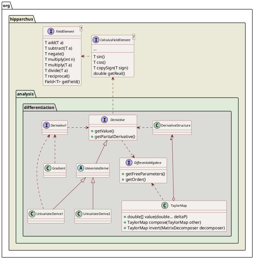
The UnivariateDerivative1 class is an implementation devoted to univariate functions and when only first order derivative is needed. This means instances of this class only holds \(f\) and \(\partial f / \partial x\). It is therefore equivalent to DerivativeStructure configured with parameters=1 and order=1. It is faster, has a simpler API, and does not need a factory.
The UnivariateDerivative2 class is an implementation devoted to univariate functions and when only first and second order derivatives are needed. This means instances of this class only holds \(f\), \(\partial f / \partial x\) and \(\partial^2 f / \partial x^2\). It is therefore equivalent to DerivativeStructure configured with parameters=1 and order=2. It is faster, has a simpler API, and does not need a factory.
The Gradient class is an implementation devoted to multivariate functions and when only first order derivatives with respect to all parameters are needed. This means instances of this class only holds \(f\), \(\partial f / \partial p_1\), \(\partial f / \partial p_2\)… \(\partial f / \partial p_n\). It is therefore equivalent to DerivativeStructure configured with parameters=n and order=1. It is faster, has a simpler API, and does not need a factory.
There are field versions of all these classes: FieldUnivariateDerivative1, FieldUnivariateDerivative2, FieldGradient.
Differentiable functions
There are several ways a user can create an implementation of the UnivariateDifferentiableFunction interface. The first method is to simply write it directly using the appropriate methods from DerivativeStructure to compute addition, subtraction, sine, cosine… This is often quite straigthforward and there is no need to remember the rules for differentiation: the user code only represents the function itself, the differentials will be computed automatically under the hood. The second method is to write a classical UnivariateFunction and to pass it to an existing implementation of the UnivariateFunctionDifferentiator interface to retrieve a differentiated version of the same function. The first method is more suited to small functions for which the user already controls all the underlying code. The second method is better suited to either large functions that would be cumbersome to write using the DerivativeStructure API, or functions for which the user does not have control over the full underlying code (for example functions that call external libraries).
Hipparchus provides one implementation of the UnivariateFunctionDifferentiator interface: FiniteDifferencesDifferentiator. This class creates a wrapper that will call the user-provided function on a grid sample and will use finite differences to compute the derivatives. It takes care of boundaries if the variable is not defined on the whole real line. It is possible to use more points than strictly required by the derivation order (for example one can specify an 8-points scheme to compute first derivative only). However, one must be aware that tuning the parameters for finite differences is highly problem-dependent. Choosing the wrong step size or the wrong number of sampling points can lead to huge errors. Finite differences are also not well suited to compute high order derivatives. Here is an example on how this implementation can be used:
// function to be differentiated
UnivariateFunction basicF = new UnivariateFunction() {
                                public double value(double x) {
                                    return x * FastMath.sin(x);
                                }
                            });

// create a differentiator using 5 points and 0.01 step
FiniteDifferencesDifferentiator differentiator =
    new FiniteDifferencesDifferentiator(5, 0.01);

// create a new function that computes both the value and the derivatives
// using DerivativeStructure
UnivariateDifferentiableFunction completeF = differentiator.differentiate(basicF);

// now we can compute display the value and its derivatives
// here we decided to display up to second order derivatives,
// because we feed completeF with order 2 DerivativeStructure instances
DSFactory factory = new DSFactory(1, 2);
for (double x = -10; x < 10; x += 0.1) {
    DerivativeStructure xDS = factory.variable(0, x);
    DerivativeStructure yDS = f.value(xDS);
    System.out.format(Locale.US, "%7.3f %7.3f %7.3f%n",
                      yDS.getValue(),
                      yDS.getPartialDerivative(1),
                      yDS.getPartialDerivative(2));
}
Note that using FiniteDifferencesDifferentiator in order to have a UnivariateDifferentiableFunction that can be provided to a Newton-Raphson's solver is a very bad idea. The reason is that finite differences are not really accurate and need lots of additional calls to the basic underlying function. If the user initially has only the basic function available and needs to find its roots, it is much more accurate and much more efficient to use a solver that only requires the function values and not the derivatives. A good choice is to use bracketing n method, which in fact converges faster than Newton-Raphson's and can be configured to a higher order (typically 5) than Newton-Raphson which is an order 2 method.
Another implementation of the UnivariateFunctionDifferentiator interface is under development in the related project Apache Commons Nabla. This implementation uses automatic code analysis and generation at binary level. However, at time of writing (end 2012), this project is not yet suitable for production use.